Individual Conditional Expectation (ICE)

(Feature Influence)

Kacper Sokol

Topics

• Method Overview
• (Algorithmic) Building Blocks
• Theoretical Underpinning
• Variants
• Examples
• Case Studies & Gotchas!
• Properties
• Further Considerations

Method Overview

Explanation Synopsis

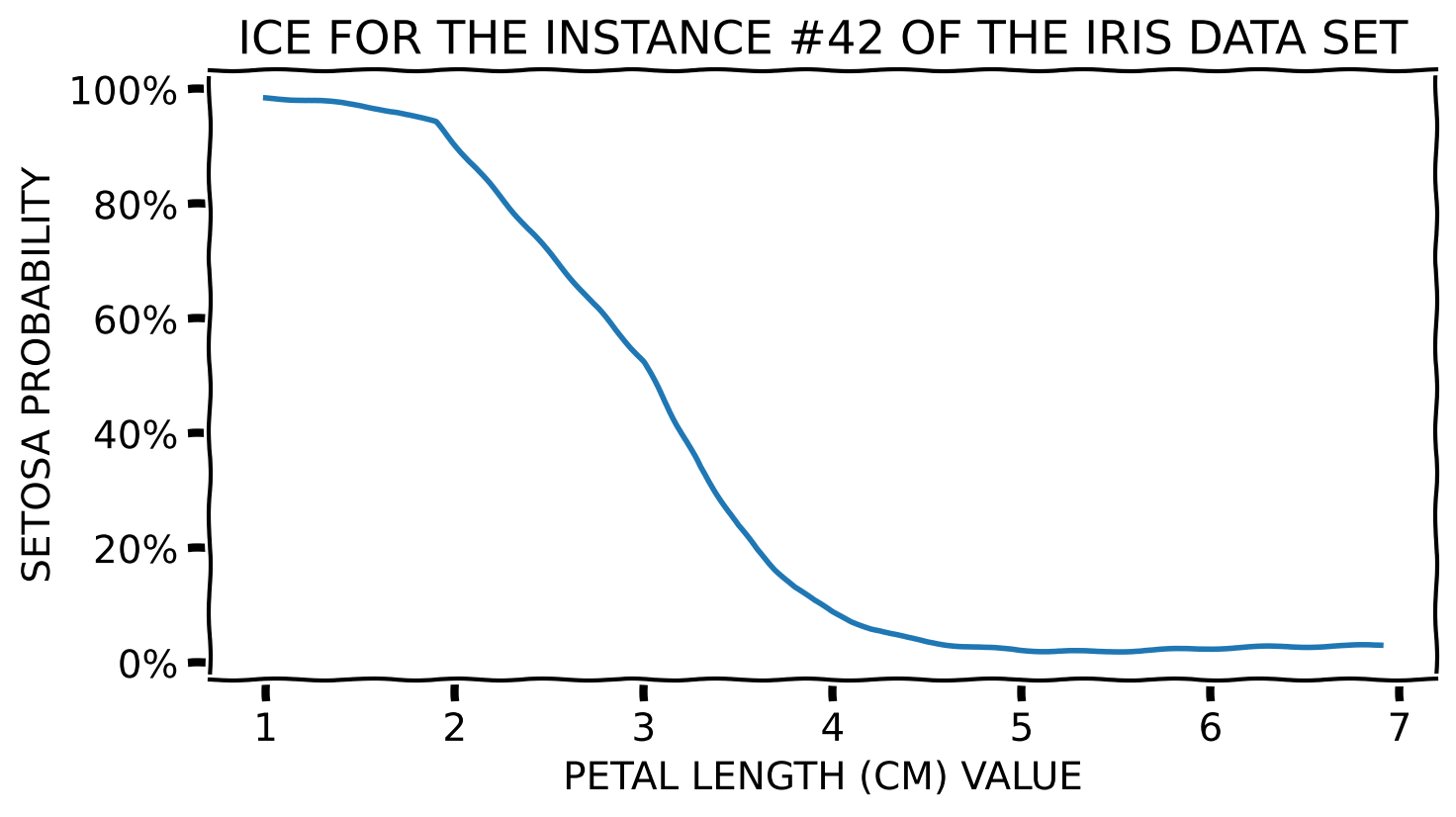
ICE captures the response of a predictive model for a single instance when varying one of its features (Goldstein et al. 2015).

It communicates local (with respect to a single instance) feature influence.

Toy Example – Numerical Feature

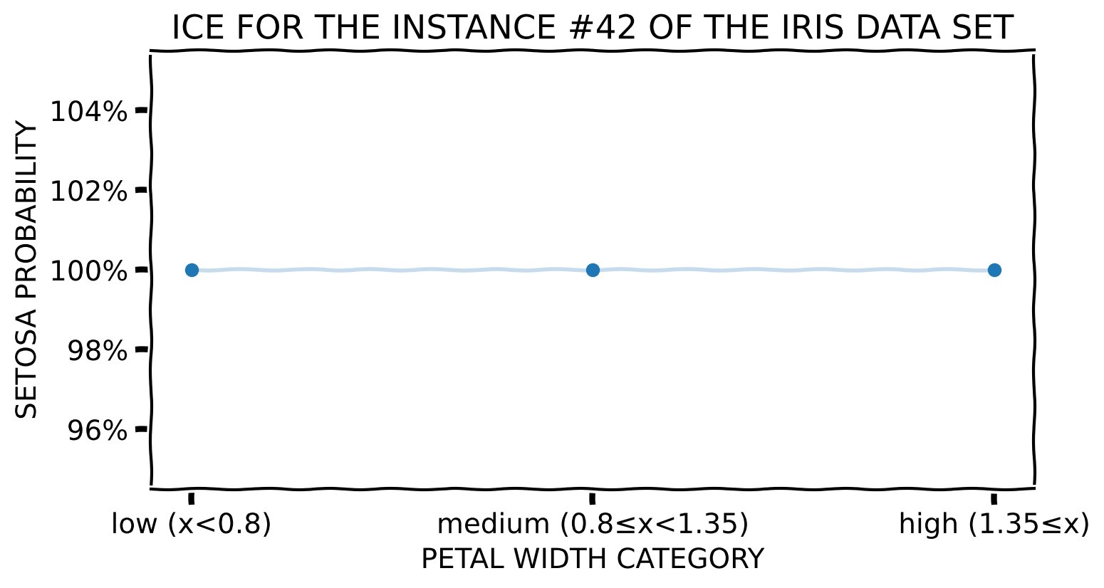
Toy Example – Categorical Feature

• The lines don’t show trajectories as these are meaningless for unordered categories.
• The lines are only useful to discern changes for individual instances.

Method Properties

Property	Individual Conditional Expectation
relation	post-hoc
compatibility	model-agnostic
modelling	regression, crisp and probabilistic classification
scope	local (per instance; generalises to cohort or global)
target	prediction (generalises to model)

Method Properties    

Property	Individual Conditional Expectation
data	tabular
features	numerical and categorical
explanation	feature influence (visualisation)
caveats	feature correlation, unrealistic instances

(Algorithmic) Building Blocks

Computing ICE

Input

1. Select a feature to explain

2. Select the explanation target

   • crisp classifiers → one-vs.-the-rest or all classes
   • probabilistic classifiers → (probabilities of) one class
   • regressors → numerical values

3. Select an instance to be explained (or collection thereof)

Computing ICE    

Parameters

1. Define granularity of the explained feature

   • numerical attributes → select the range – minimum and maximum value – and the step size of the feature
   • categorical attributes → the full set or a subset of possible values

Computing ICE    

Procedure

1. For each explained instance create its copy with the value of the explained feature replaced by the range of values determined by the explanation granularity
2. Predict the augmented data
3. For each explained instance plot a line that represents the response of the explained model across the entire spectrum of the explained feature

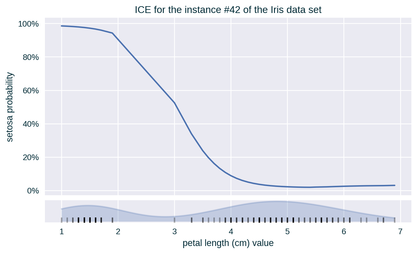
    Since the values of the explained feature may not be uniformly distributed in the underlying data set, a rug plot showing the distribution of its feature values can help in interpreting the explanation.

Theoretical Underpinning

Formulation    

\[ X_{\mathit{ICE}} \subseteq \mathcal{X} \]

\[ V_i = \{ v_i^{\mathit{min}} , \ldots , v_i^{\mathit{max}} \} \]

\[ f \left( x_{\setminus i} , x_i=v_i \right) \;\; \forall \; x \in X_{\mathit{ICE}} \; \forall \; v_i \in V_i \]

\[ f \left( x_{\setminus i} , x_i=V_i \right) \;\; \forall \; x \in X_{\mathit{ICE}} \]

Formulation        

Original notation (Goldstein et al. 2015)

\[ \left\{ \left( x_{S}^{(i)} , x_{C}^{(i)} \right) \right\}_{i=1}^N \]

\[ \hat{f}_S^{(i)} = \hat{f} \left( x_{S}^{(i)} , x_{C}^{(i)} \right) \]

• \(x_S\) is stepped through – the explained feature
• \(x_C\) are the given feature values

Variants

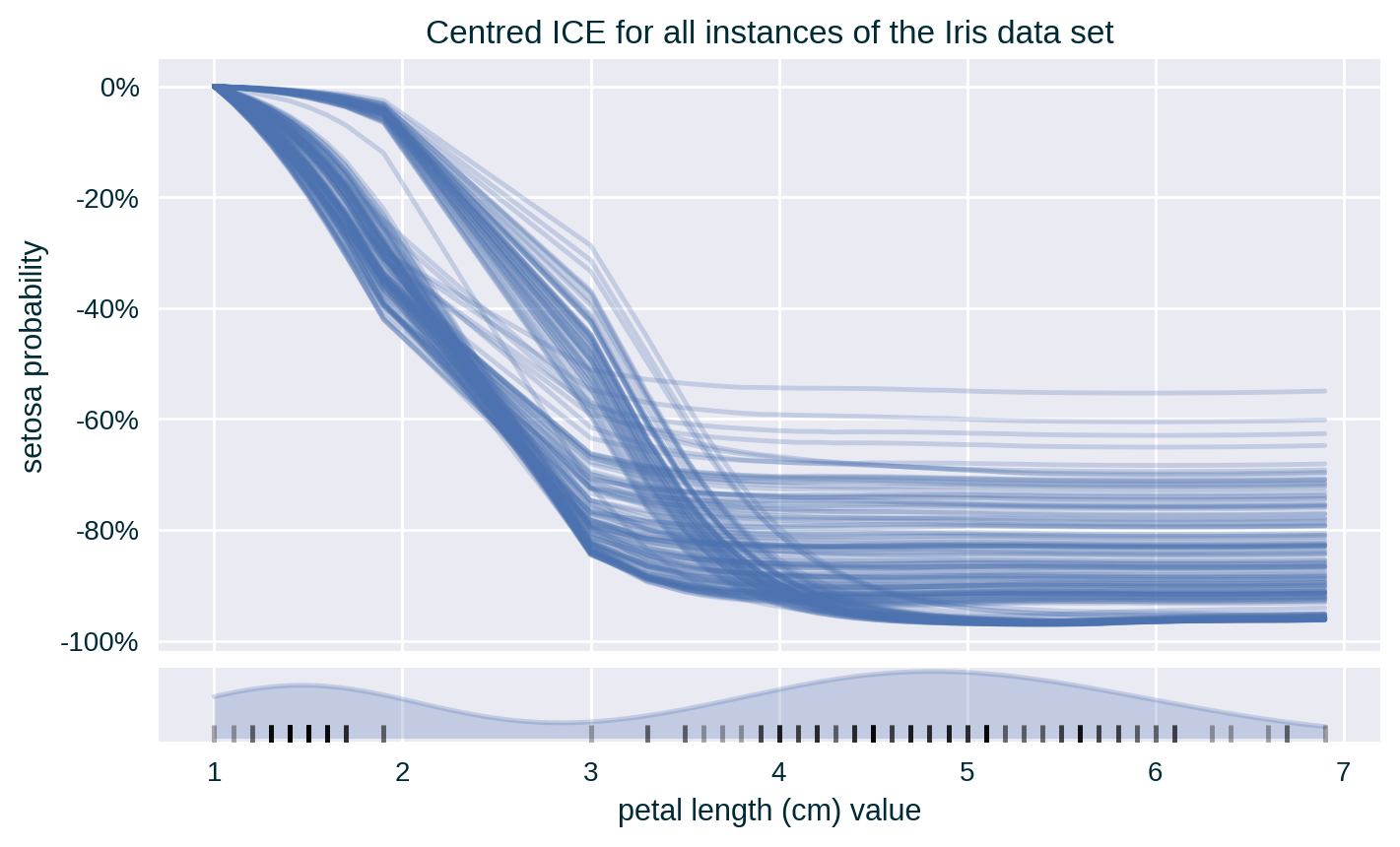
Centred ICE

Centres ICE curves by anchoring them at a fixed point, usually the lower end of the explained feature range.

\[ f \left( x_{\setminus i} , x_i=V_i \right) - f \left( x_{\setminus i} , x_i=v_i^{\mathit{min}} \right) \;\; \forall \; x \in X_{\mathit{ICE}} \]

or

\[ \hat{f} \left( x_{S}^{(i)} , x_{C}^{(i)} \right) - \hat{f} \left( x^{\star} , x_{C}^{(i)} \right) \]

Helps to see whether the ICE curves of individual instances behave differently.

Derivative ICE

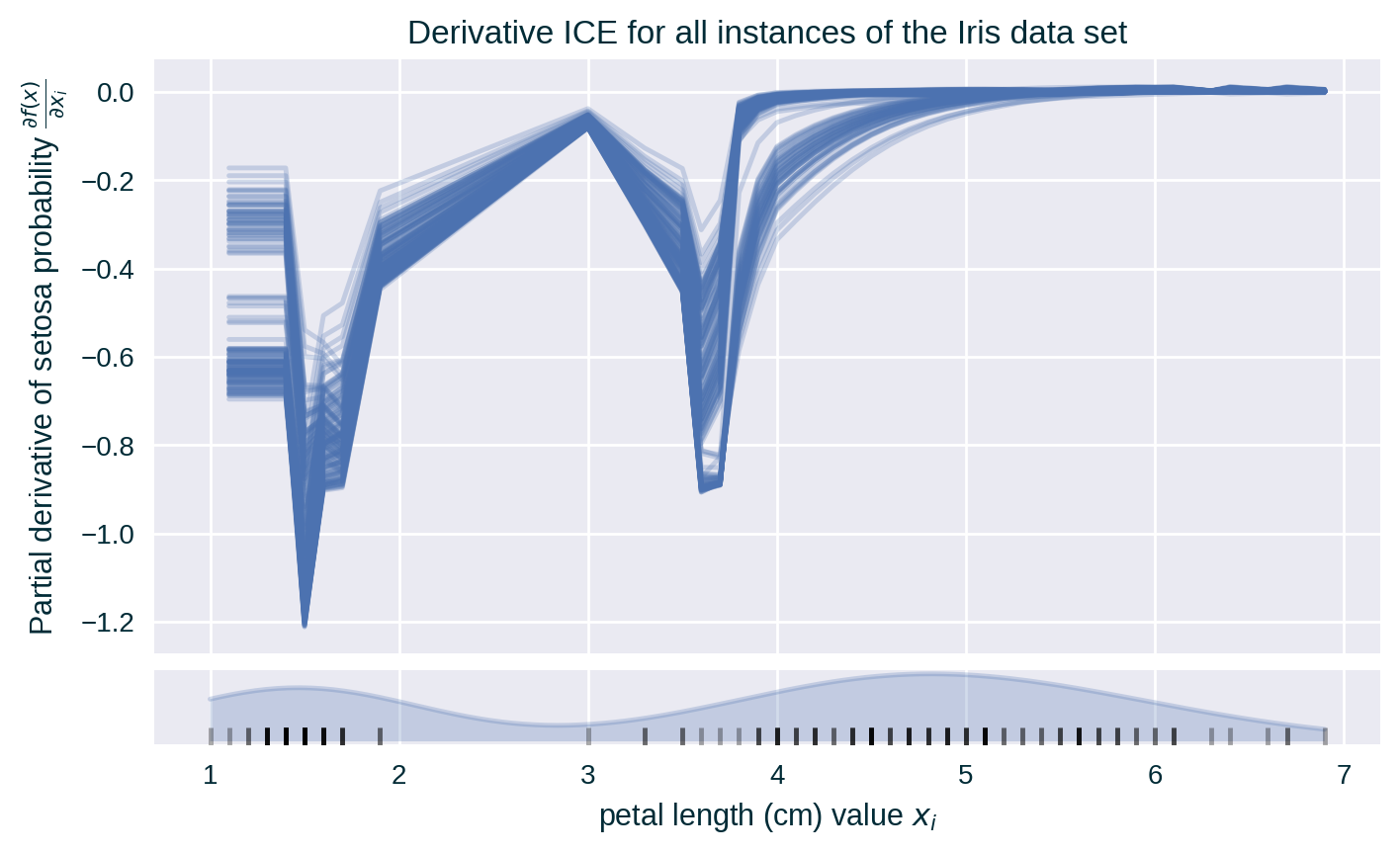
Visualises interaction effects between the explained and remaining features by calculating the partial derivative of the explained model \(f\) with respect to the explained feature \(x_i\).

• When no interactions are present, all curves overlap.
• When interactions exist, the lines will be heterogeneous.

Derivative ICE    

\[ f \left( x_{\setminus i} , x_i \right) = g \left( x_i \right) + h \left( x_{\setminus i} \right) \;\; \text{so that} \;\; \frac{\partial f(x)}{\partial x_i} = g^\prime(x_i) \]

or

\[ \hat{f} \left( x_{S} , x_{C} \right) = g \left( x_{S} \right) + h \left( x_{C} \right) \;\; \text{so that} \;\; \frac{\partial \hat{f}(x)}{\partial x_{S}} = g^\prime(x_{S}) \]

• This assumes no interaction (correlation) between the inspected / explained and the remaining features.
• (Derivatives) communicates the rate and direction of changes in each ICE line.

Examples

ICE of a Single Instance

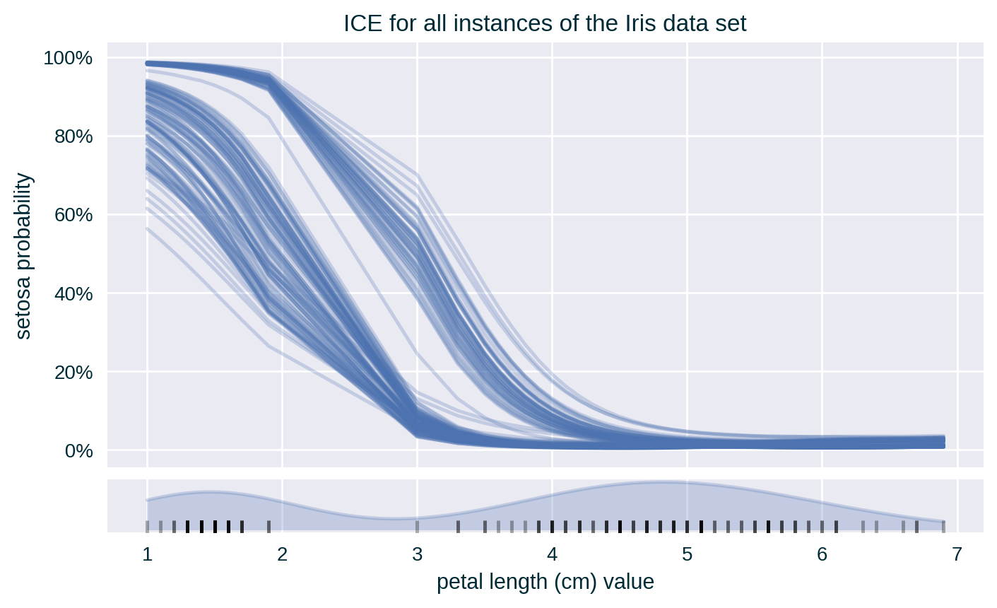
ICE of a Data Collection

Centred ICE

Derivative ICE

Case Studies & Gotchas!

Out-of-distribution (Impossible) Instances

Out-of-distribution (Impossible) Instances    

Out-of-distribution (Impossible) Instances    

Note the gaps in the feature range, which is due to how scikit-learn computes the range for ICE calculation.

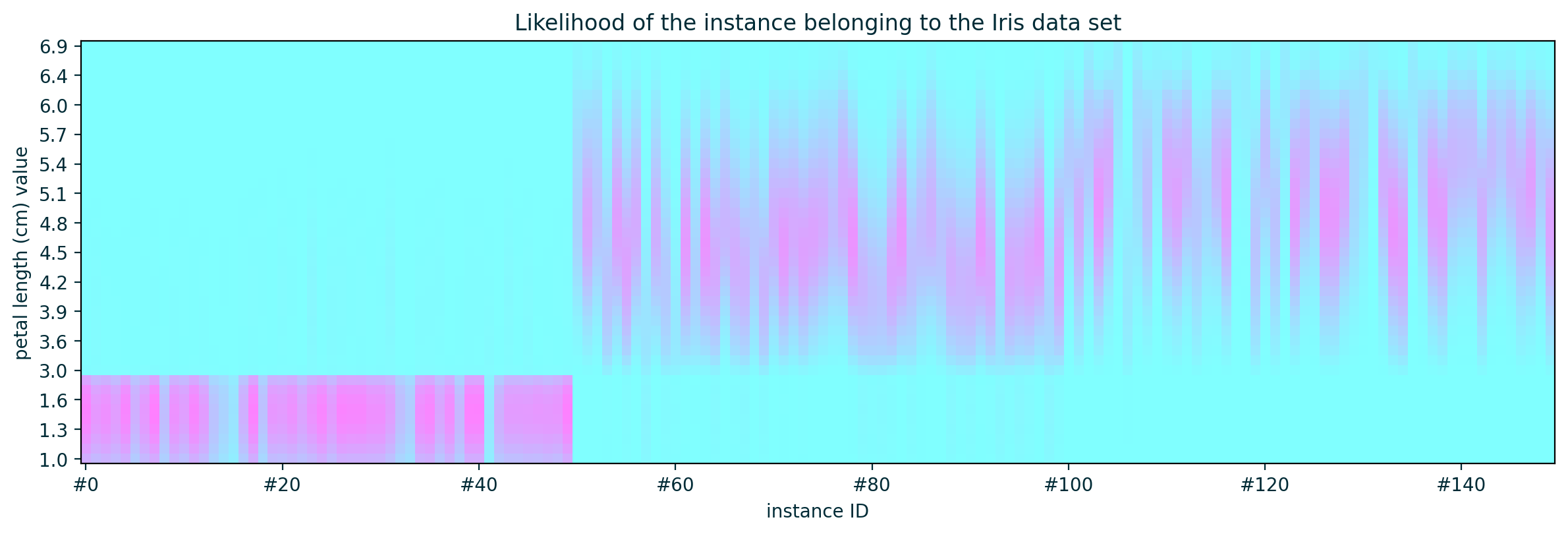
Out-of-distribution (Impossible) Instances    

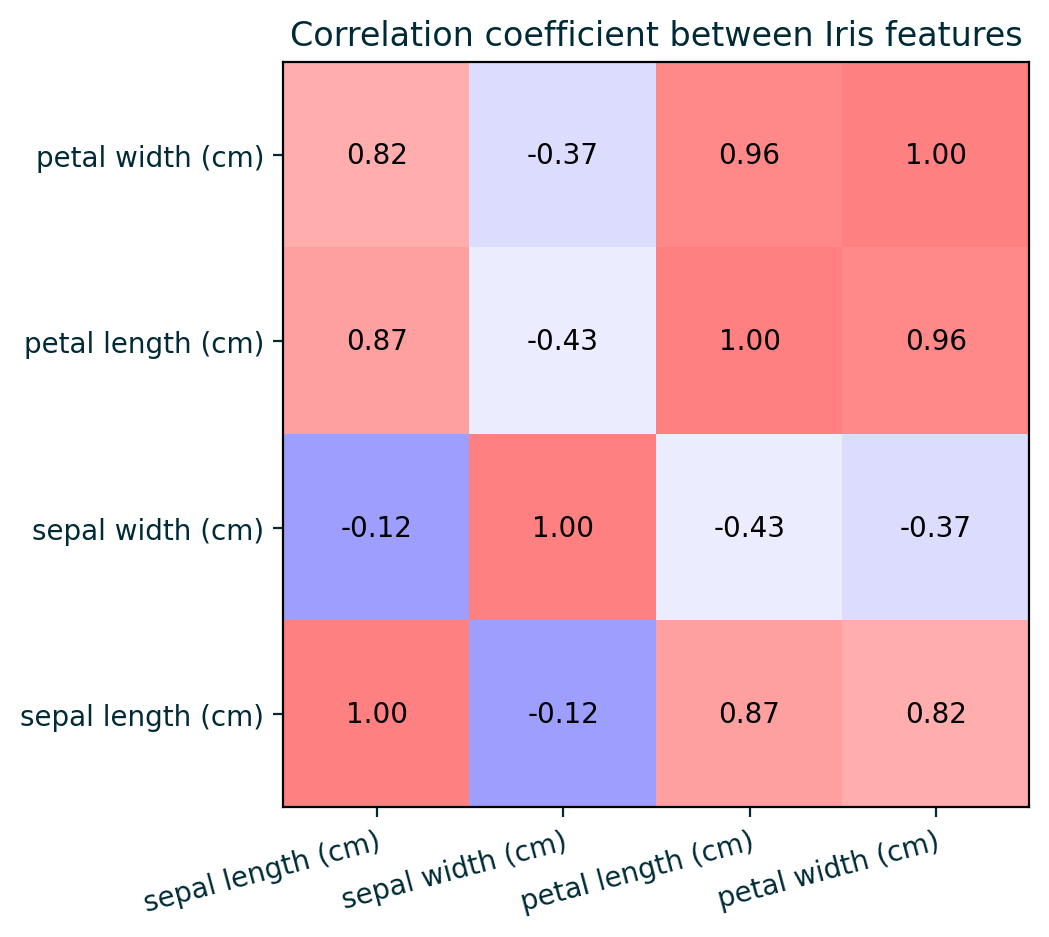
Feature Correlation

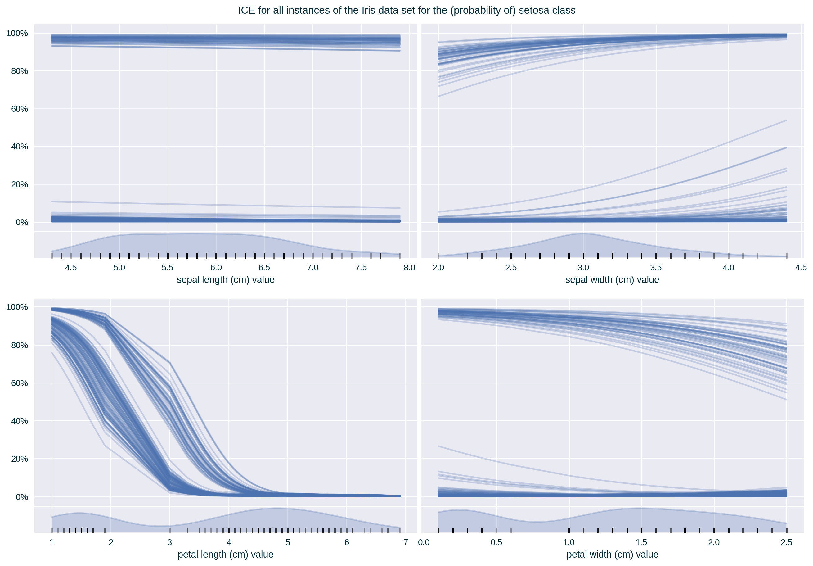
Feature Correlation    

• Go back to the previous plot and show that for negative coefficient features the probability decreases; but for positive coefficient features it increases.
• The rate of chagne depends on the magnitude of the coefficient.
• Caveat: The features were not normalised to the same range so these aren’t really directly comparable.

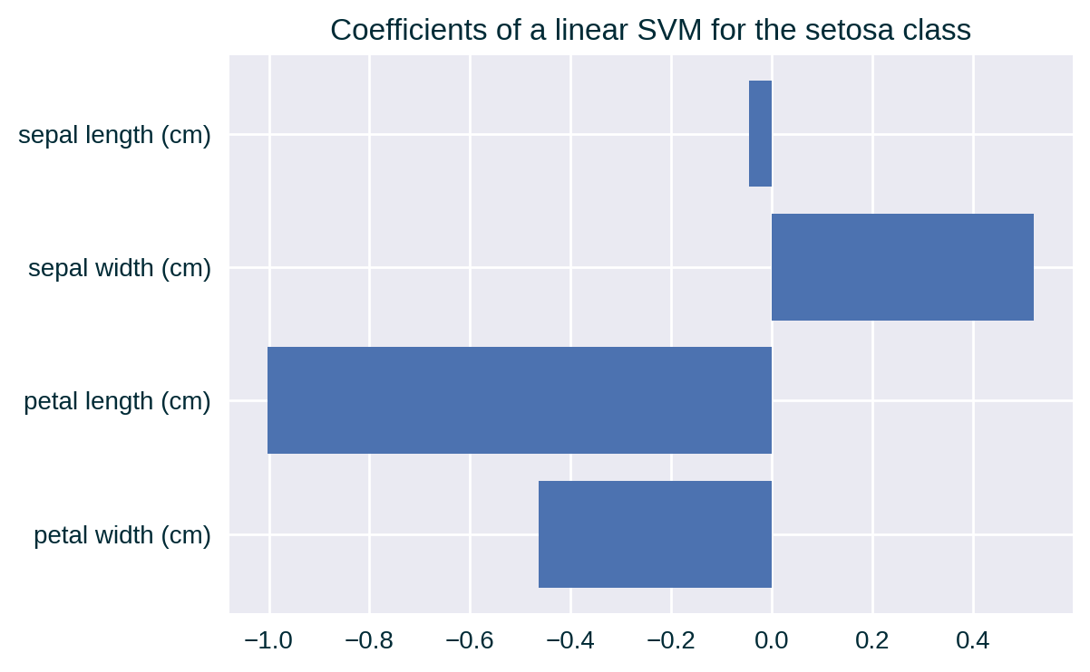
Feature Correlation    

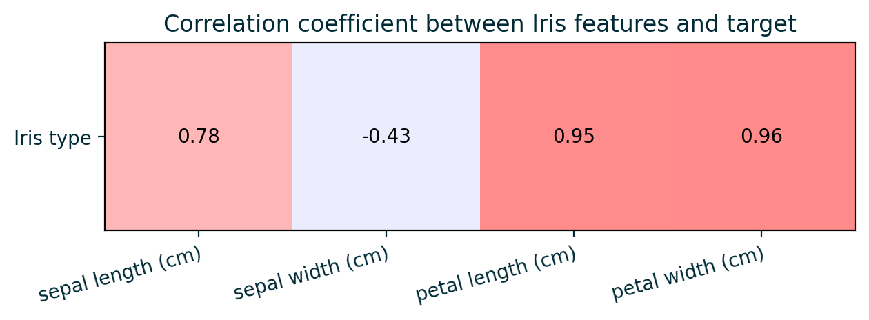
Target Correlation

Feature 2 & 1 Correlation (small)

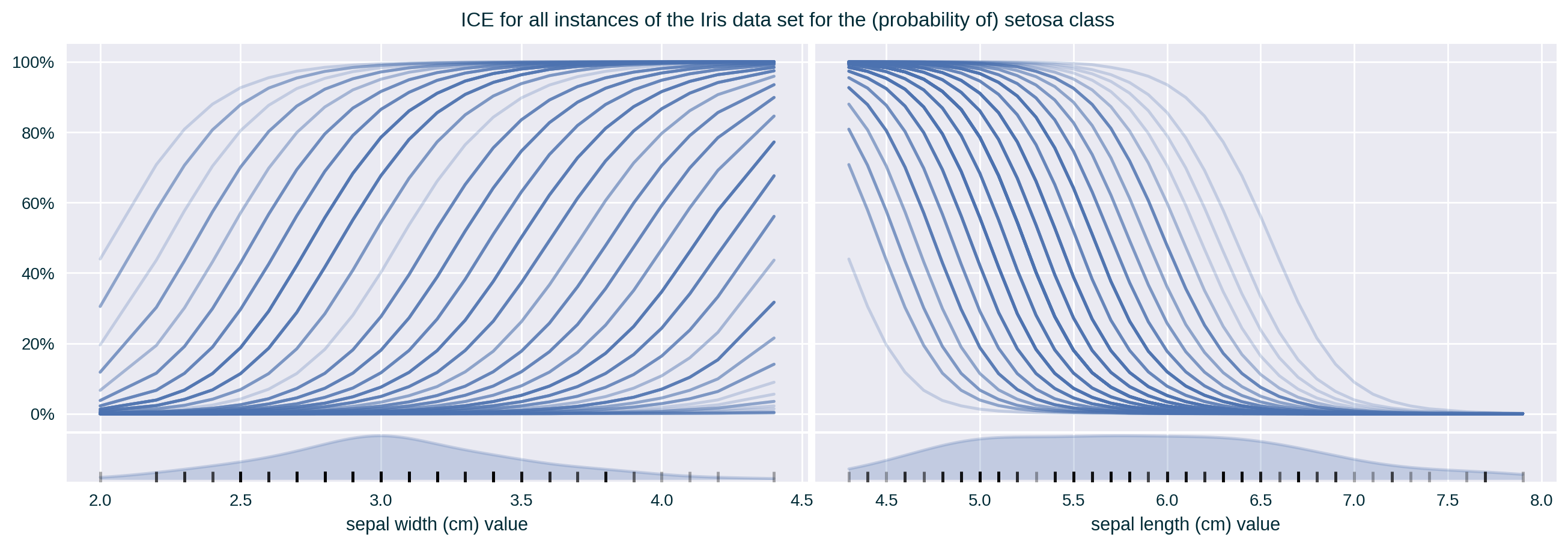
Feature 2 & 1 Correlation (small)    

• When using the features with least correlation, the behaviour is most unlike the full 4 feature plot.
• As we will see with the other (correlated) figures, the behaviour is almost unchanged.

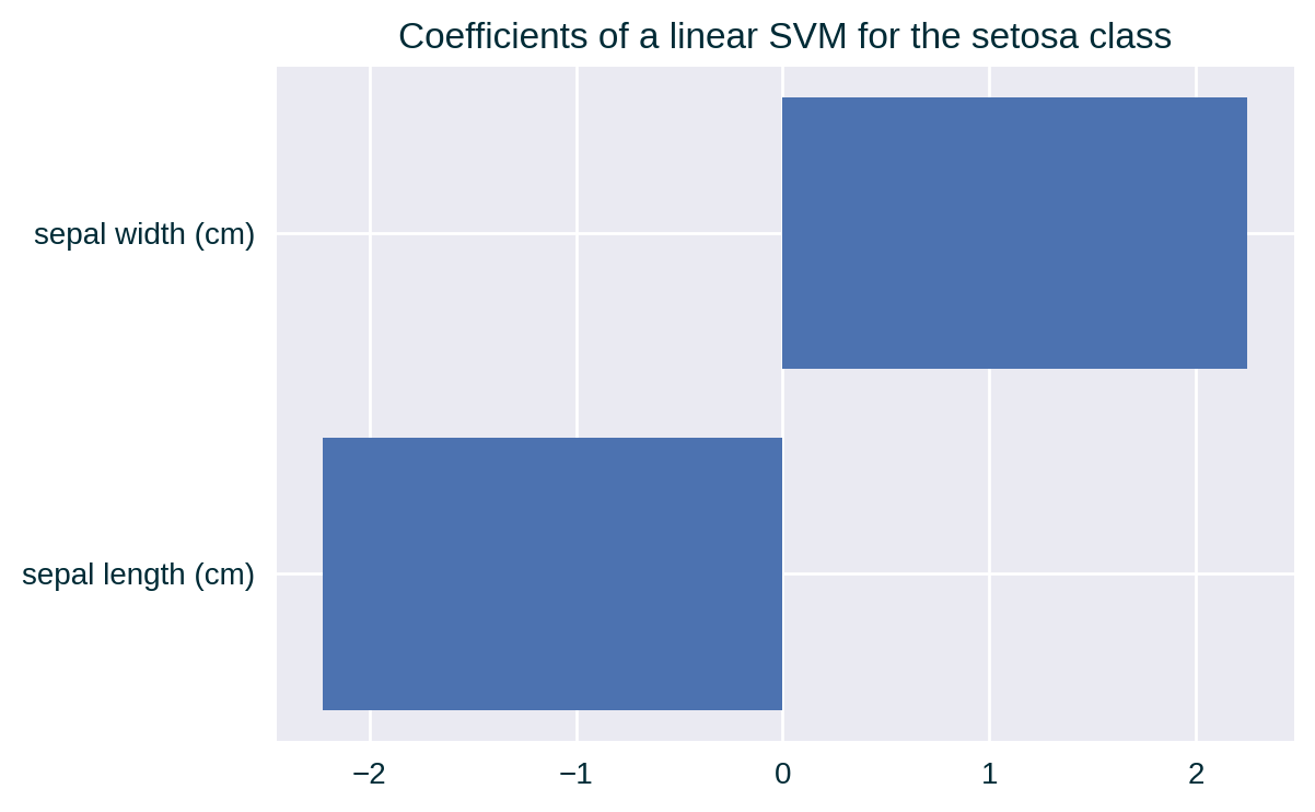
Feature 2 & 3 Correlation (medium)

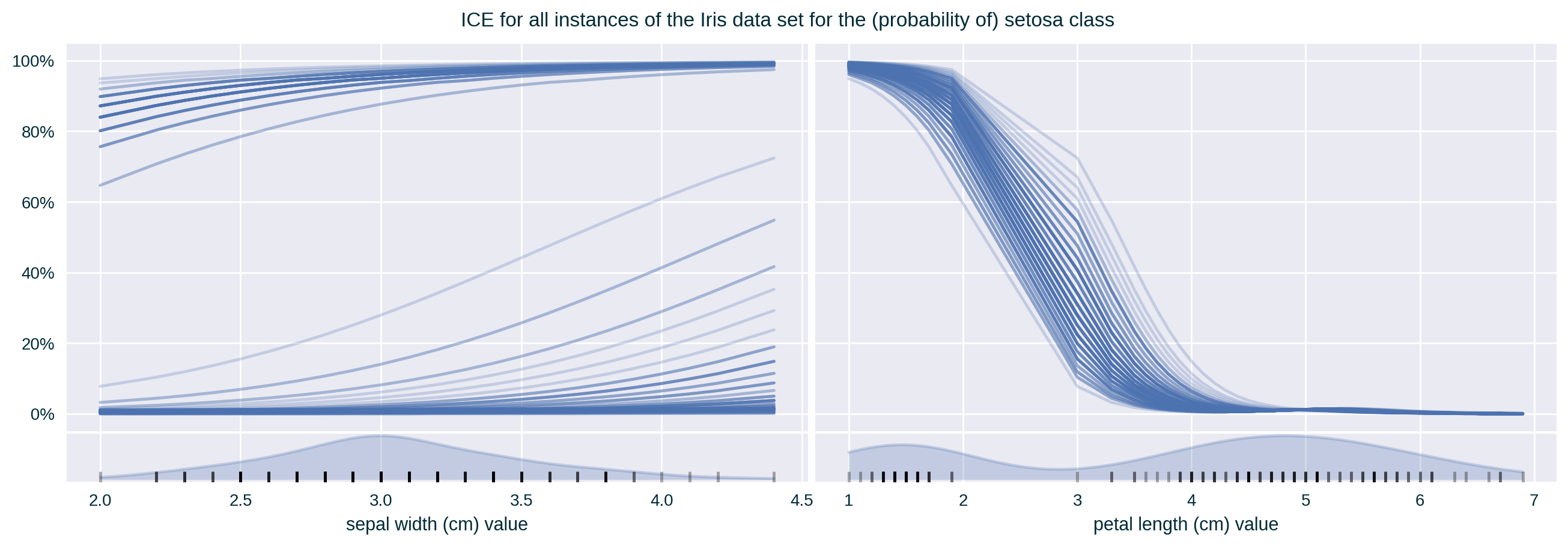
Feature 2 & 3 Correlation (medium)    

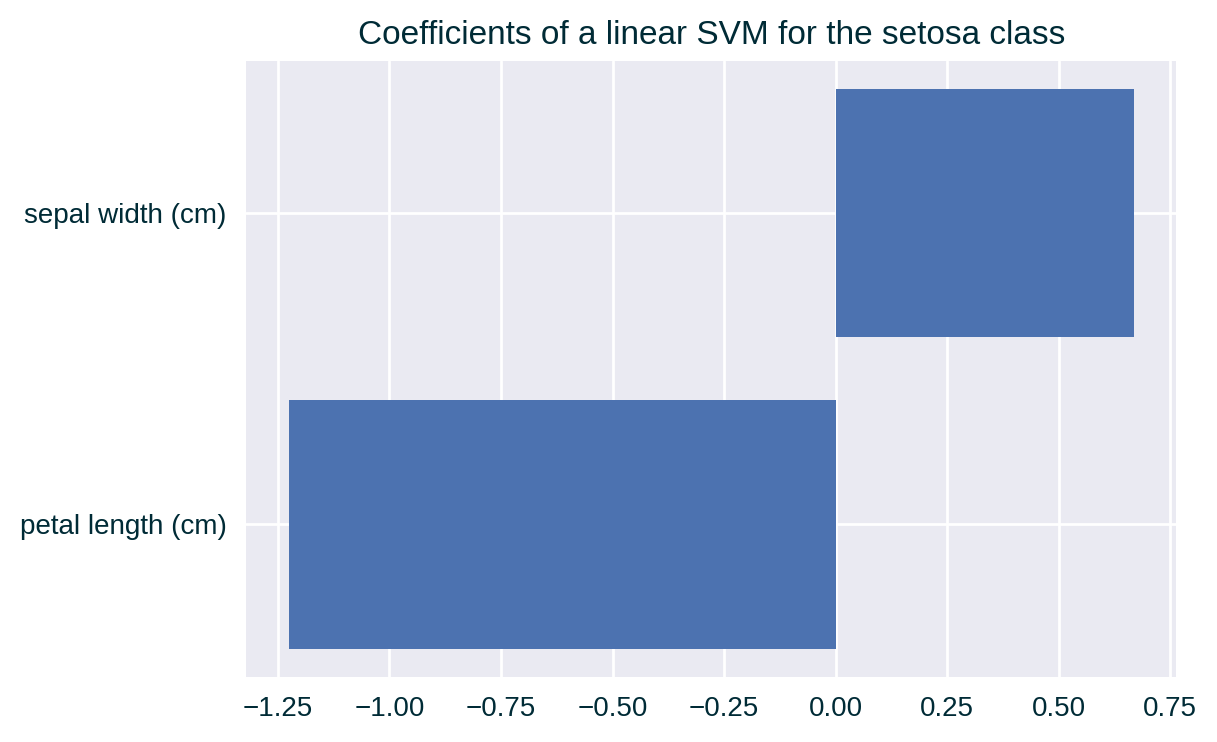
Feature 2 & 4 Correlation (medium)

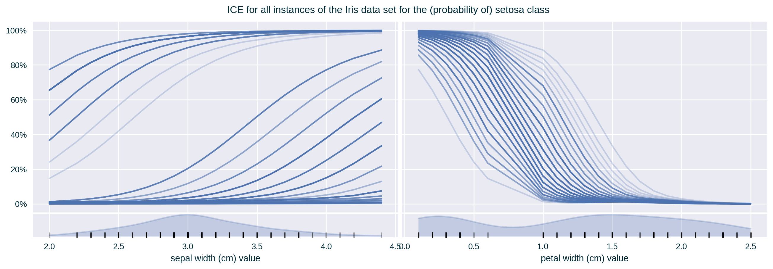
Feature 2 & 4 Correlation (medium)    

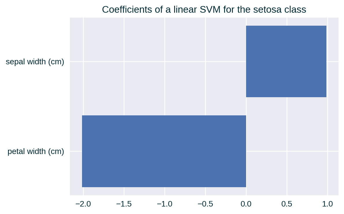
Feature 3 & 4 Correlation (high)

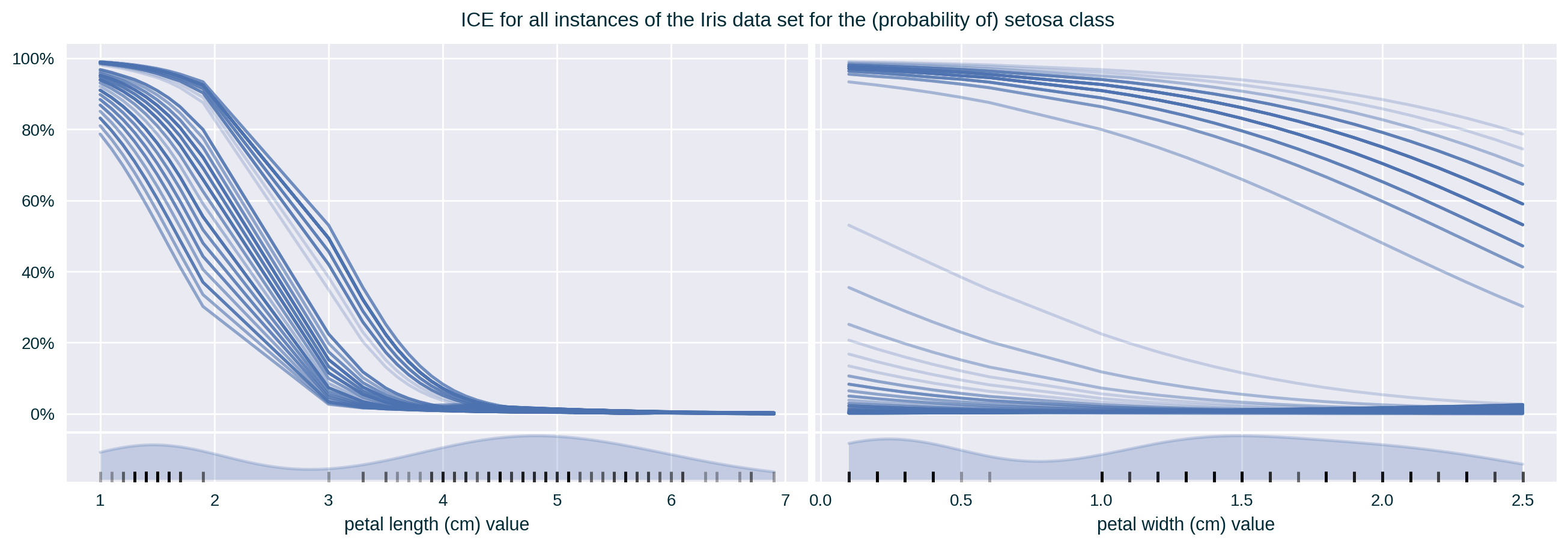
Feature 3 & 4 Correlation (high)    

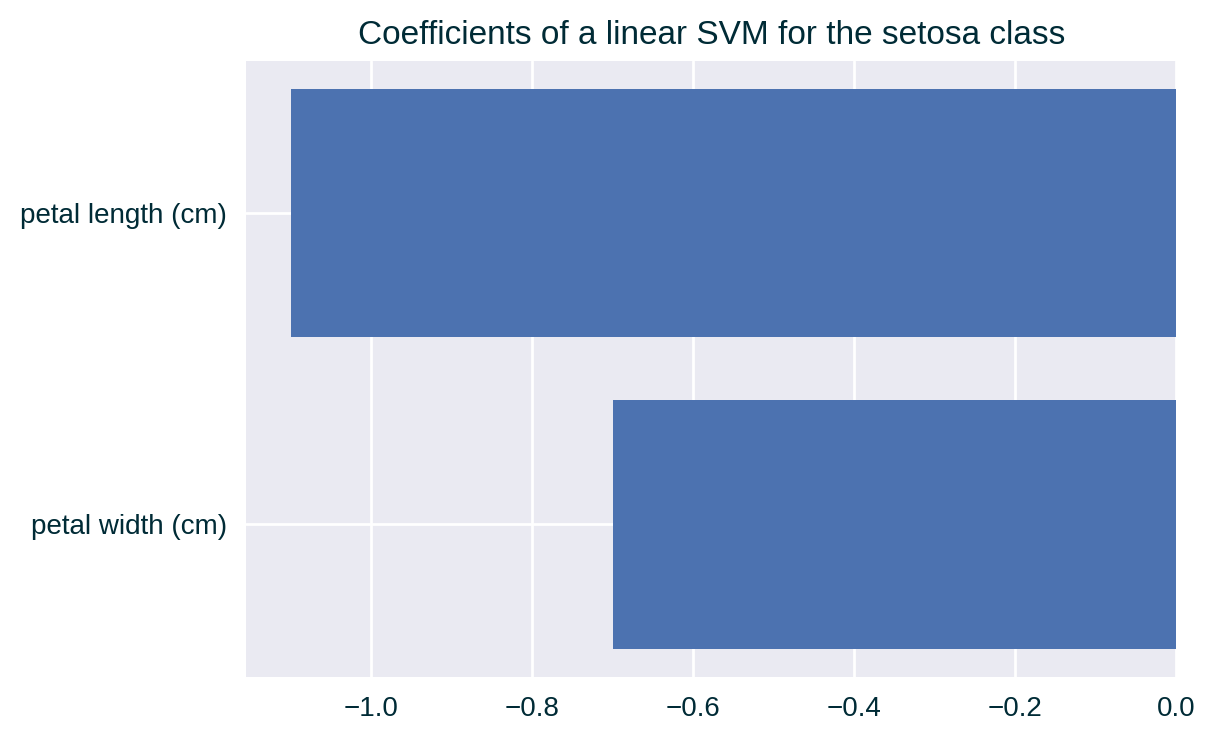
Properties

Pros    

• Easy to generate and interpret
• Spanning multiple instances allows to capture the diversity (heterogeneity) of the model’s behaviour

Cons    

• Assumes feature independence, which is often unreasonable
• ICE may not reflect the true behaviour of the model since it displays the behaviour of the model for unrealistic instances
• May be unreliable for certain values of the explained feature when its values are not uniformly distributed (abated by a rug plot)
• Limited to explaining one feature at a time

Caveats    

• Averaging ICEs gives Partial Dependence (PD)
• Generating ICEs may be computationally expensive for large sets of data and wide feature intervals with a small “inspection” step
• Computational complexity: \(\mathcal{O} \left( n \times d \right)\), where
  • \(n\) is the number of instances in the designated data set and
  • \(d\) is the number of steps within the designated feature interval

Further Considerations

Causal Interpretation

Under certain (quite restrictive) assumptions, ICE is admissible to a causal interpretation (Zhao and Hastie 2021).

See Causal Interpretation of Partial Dependence (PD) for more detail.

Related Techniques

Partial Dependence (PD)

    Model-focused (global) “version” of Individual Conditional Expectation, which is calculated by averaging ICE across a collection of data points (Friedman 2001). It communicates the average influence of a specific feature value on the model’s prediction by fixing the value of this feature across a designated set of instances.

Related Techniques    

Marginal Effect (Marginal Plots or M-Plots)

    It communicates the influence of a specific feature value – or similar values, i.e., an interval around the selected value – on the model’s prediction by only considering relevant instances found in the designated data set. It is calculated as the average prediction of these instances.

Related Techniques    

Accumulated Local Effect (ALE)

    It communicates the influence of a specific feature value on the model’s prediction by quantifying the average (accumulated) difference between the predictions at the boundaries of a (small) fixed interval around the selected feature value (Apley and Zhu 2020). It is calculated by replacing the value of the explained feature with the interval boundaries for instances found in the designated data set whose value of this feature is within the specified range.

Implementations

Python	R
scikit-learn (>=0.24.0)	iml
PyCEbox	ICEbox
alibi	pdp
	DALEX

Further Reading

• ICE paper (Goldstein et al. 2015)
• Interpretable Machine Learning book
• scikit-learn example
• FAT Forensics example and tutorial

Bibliography

Apley, Daniel W, and Jingyu Zhu. 2020. “Visualizing the Effects of Predictor Variables in Black Box Supervised Learning Models.” Journal of the Royal Statistical Society: Series B (Statistical Methodology) 82 (4): 1059–86.

Friedman, Jerome H. 2001. “Greedy Function Approximation: A Gradient Boosting Machine.” Annals of Statistics, 1189–1232.

Goldstein, Alex, Adam Kapelner, Justin Bleich, and Emil Pitkin. 2015. “Peeking Inside the Black Box: Visualizing Statistical Learning with Plots of Individual Conditional Expectation.” Journal of Computational and Graphical Statistics 24 (1): 44–65.

Zhao, Qingyuan, and Trevor Hastie. 2021. “Causal Interpretations of Black-Box Models.” Journal of Business & Economic Statistics 39 (1): 272–81.