Marginal Effect (ME)
/Marginal Plots, M-Plots or
Local Dependence Profiles/

(Feature Influence)

Kacper Sokol

Topics

• Method Overview
• (Algorithmic) Building Blocks
• Theoretical Underpinning
• Variants
• Examples
• Case Studies & Gotchas!
• Properties
• Further Considerations

Method Overview

Explanation Synopsis

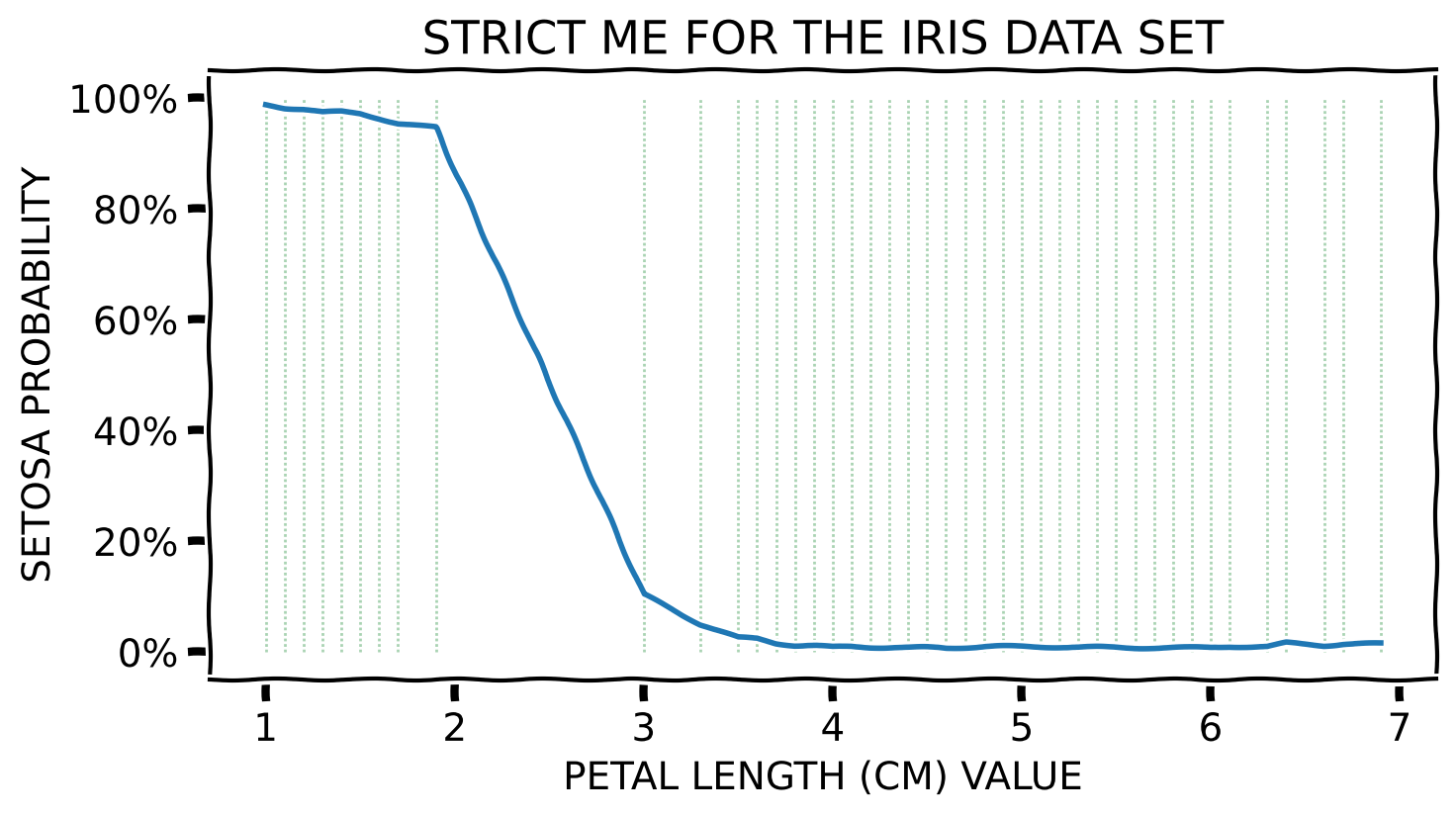
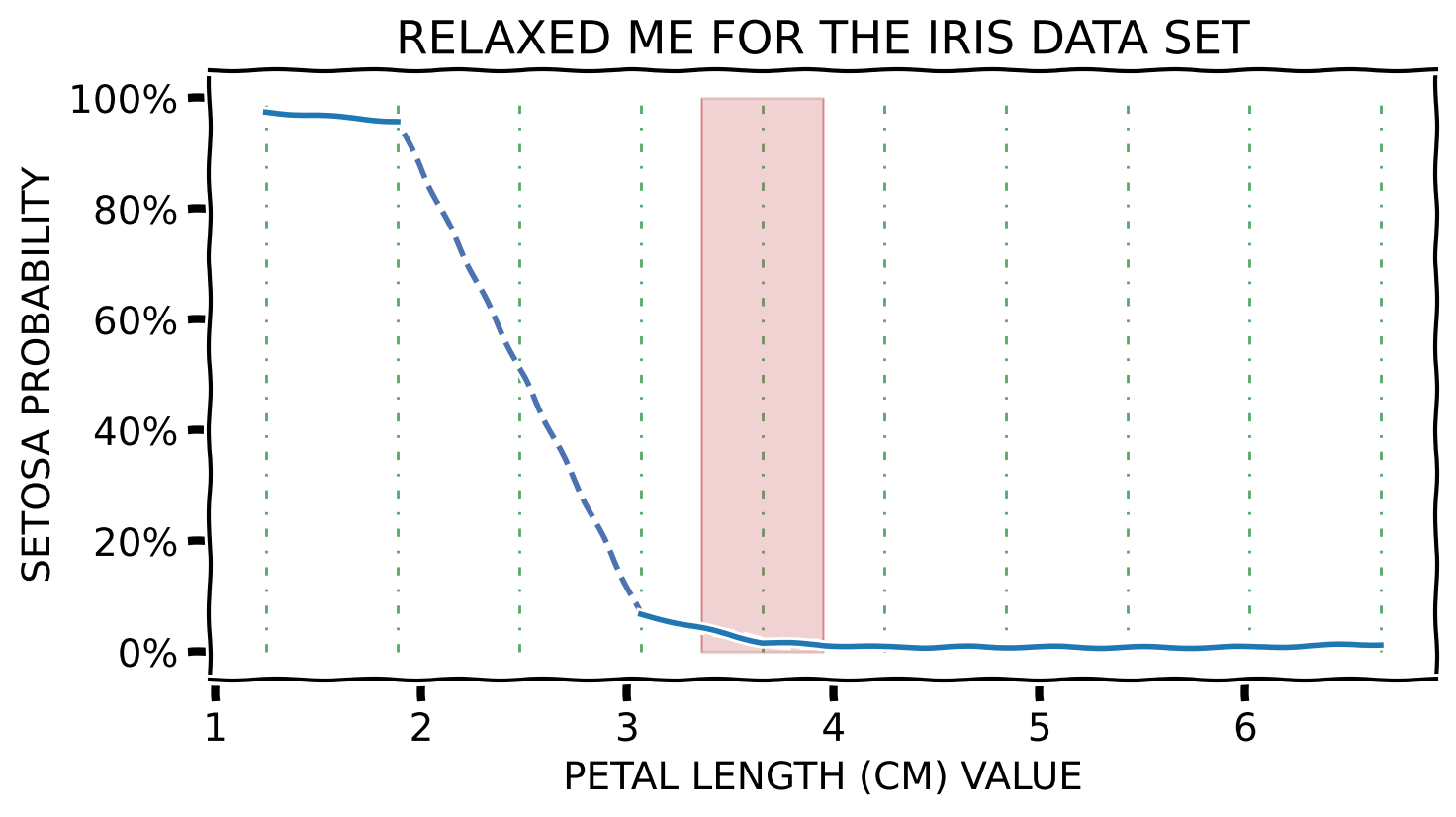
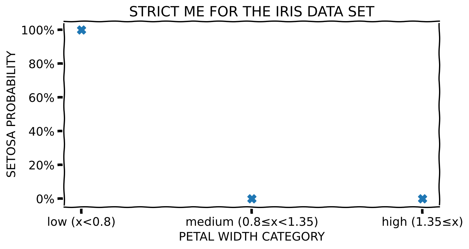
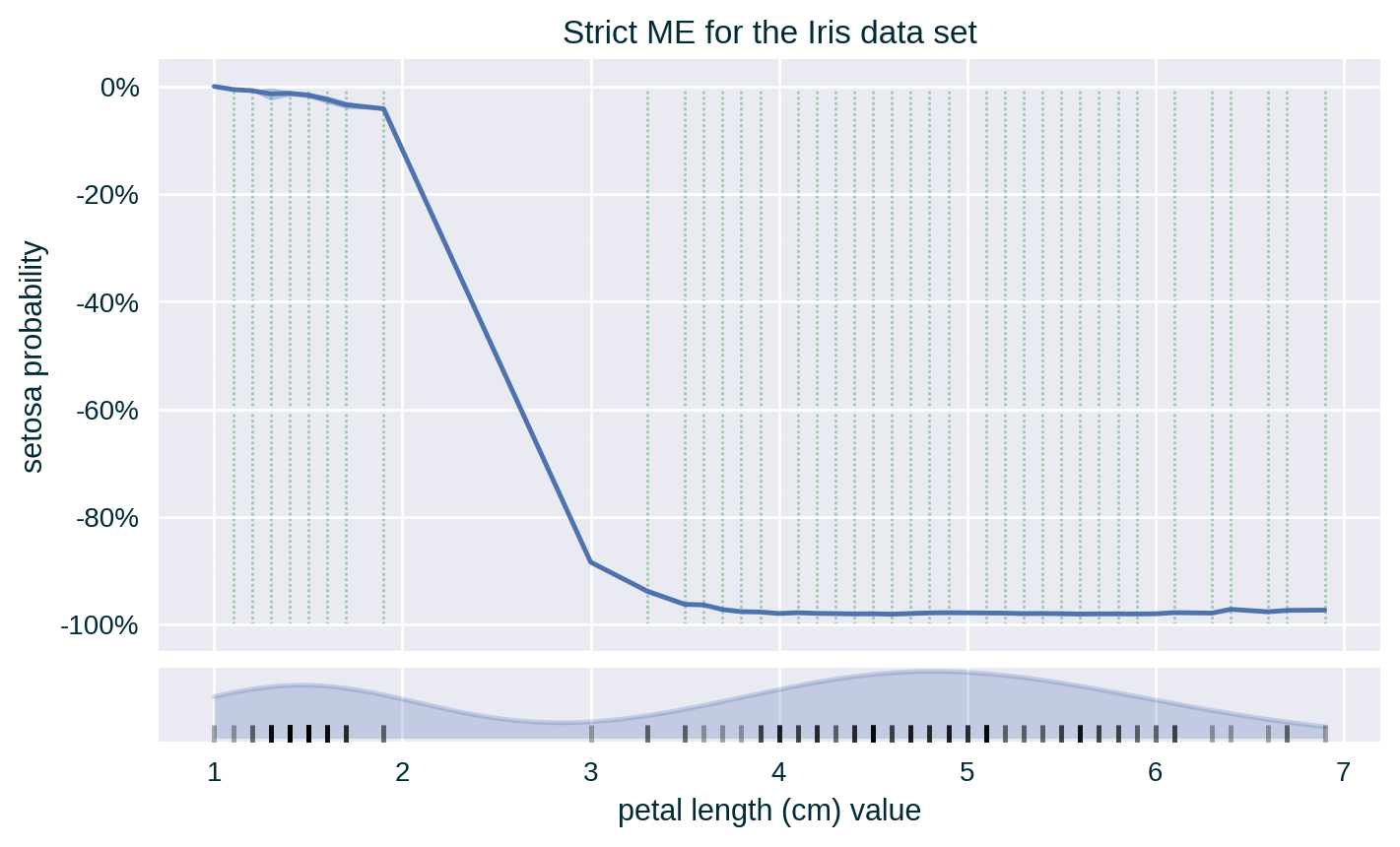
ME captures the average response of a predictive model across a collection of instances (taken from a designated data set) for a specific value of a selected feature (found in the aforementioned data set) (Apley and Zhu 2020). This measure can be relaxed by including similar feature values determined by a fixed interval around the selected value.

It communicates global (with respect to the entire explained model) feature influence.

Rationale

ME improves upon Partial Dependence (PD) (Friedman 2001) by ensuring that the influence estimates are based on realistic instances (thus respecting feature correlation), making the explanatory insights more truthful.

Method’s Name

Note that even though the Marginal Effect name suggests that these explanations are based on the marginal distribution of the selected feature, they are actually derived from its conditional distribution.

Toy Example – Strict ME – Numerical Feature

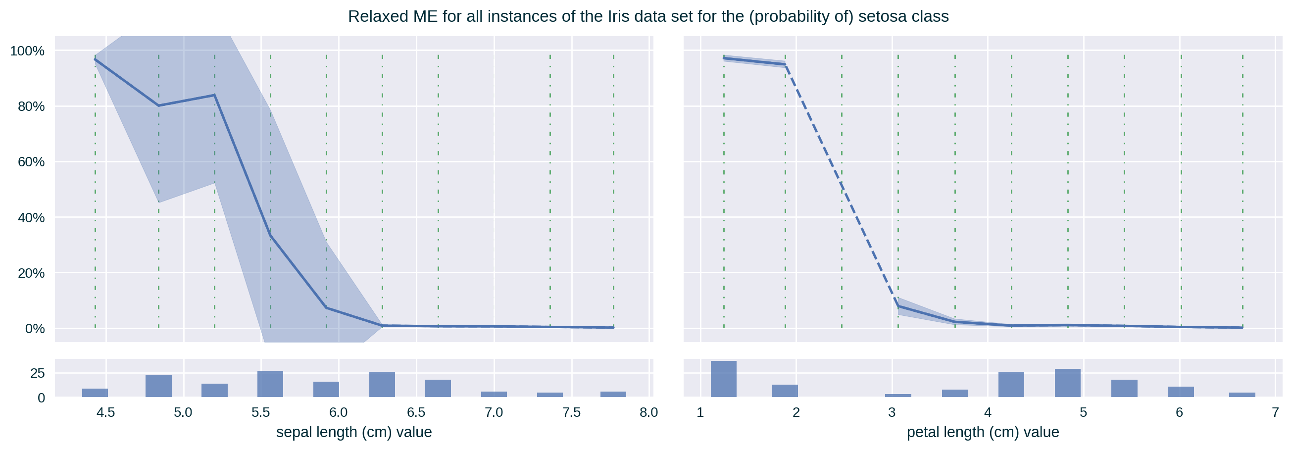
Toy Example – Relaxed ME – Numerical Feature

Toy Example – Strict ME – Categorical Feature

Method Properties

Property	Marginal Effect
relation	post-hoc
compatibility	model-agnostic
modelling	regression, crisp and probabilistic classification
scope	global (per data set; generalises to cohort)
target	model (set of predictions)

Method Properties    

Property	Marginal Effect
data	tabular
features	numerical and categorical
explanation	feature influence (visualisation)
caveats	feature correlation, heterogeneous model response

(Algorithmic) Building Blocks

Computing ME

Input

1. Select a feature to explain

2. Select the explanation target

   • crisp classifiers → one(-vs.-the-rest) or all classes
   • probabilistic classifiers → (probabilities of) one class
   • regressors → numerical values

3. Select a collection of instances to generate the explanation

Computing ME    

Parameters

1. If using the relaxed ME, define binning of the explained feature

   • numerical attributes → specify (fixed-width or quantile) binning or values of interest with a allowed variation
   • categorical attributes → the full set, a subset or grouping of possible values

Computing ME    

Procedure

1. If unavailable, collect predictions of the designated data set

2. For each instance in this set

   • for exact ME, assign it to a collection based on its value of the explained feature (possibly multiple instance per value)
   • for relaxed ME, assign it to a bin that spans the range to which the value of its explained feature belongs

3. Generate and plot Marginal Effect

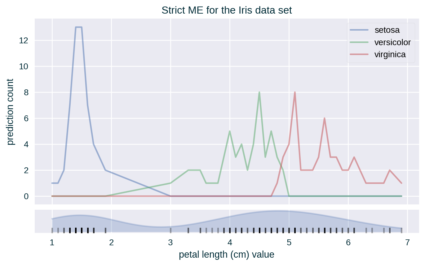
   • for crisp classifiers count the number of each unique prediction across all the instances collected for every value (exact) or bin (relaxed) of the explained feature; visualise ME either as a count or proportion using separate line for each class or using a stacked bar chart
   • for probabilistic classifiers (per class) and regressors average the response of the model across all the instances collected for each value (exact) or bin (relaxed) of the explained feature; visualise ME as a line

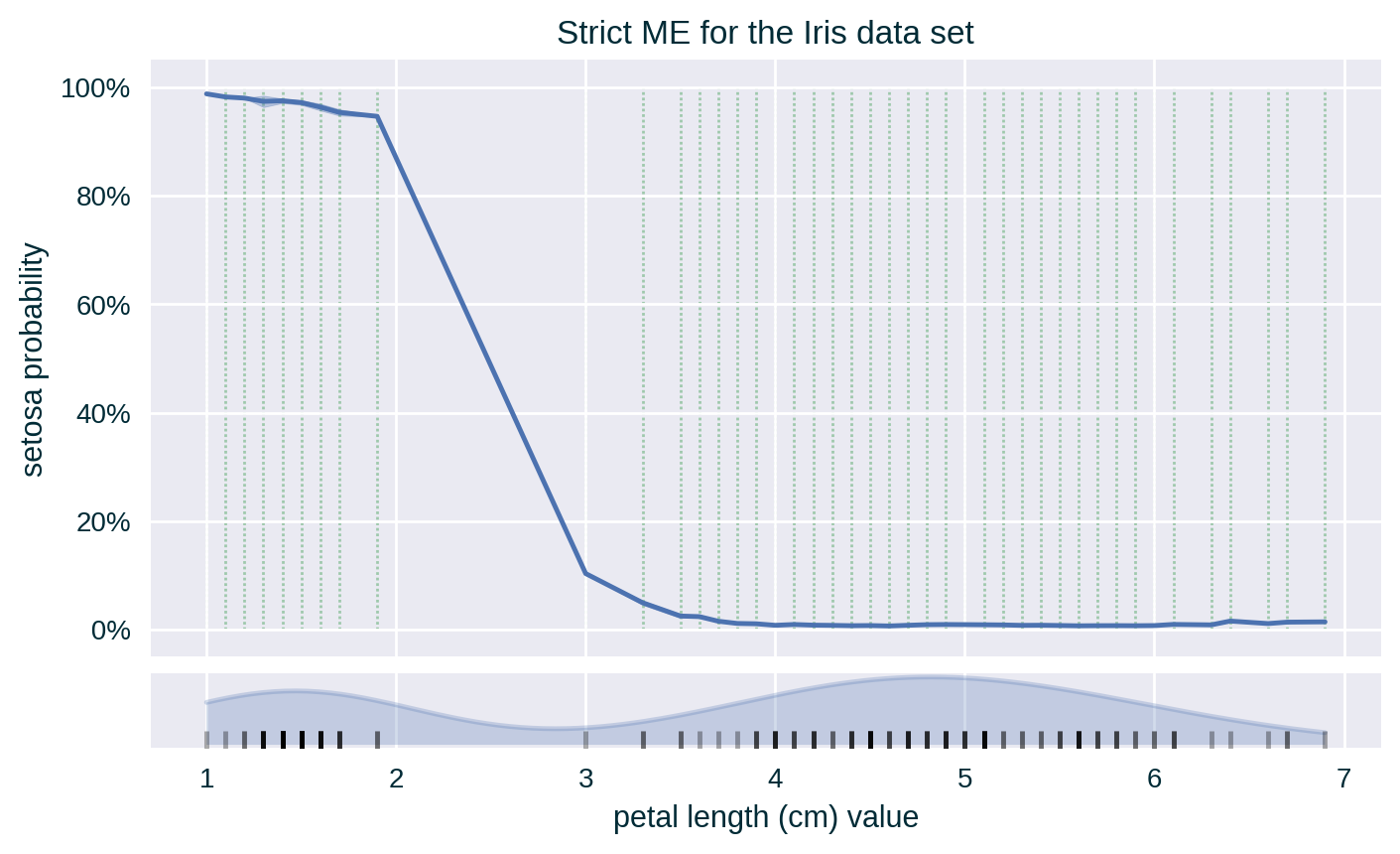
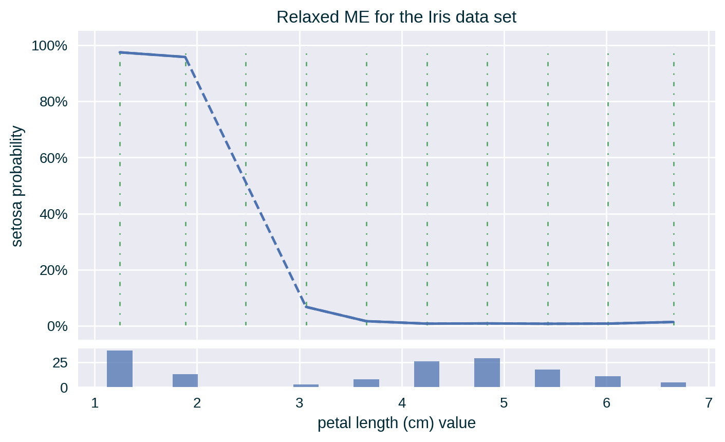
    Since the values of the explained feature may not be uniformly distributed in the underlying data set, a rug plot showing the distribution of its feature values for strict ME or a histogram representing the number of instances per bin in relaxed ME can help in interpreting the explanation.

Theoretical Underpinning

Formulation    

\[ X_{\mathit{ME}} \subseteq \mathcal{X} \]

\[ V_i = \{ x_i : x \in X_{\mathit{ME}} \} \]

\[ \mathit{ME}_i = \mathbb{E}_{X_{\setminus i} | X_{i}} \left[ f \left( X_{\setminus i} , X_{i} \right) | X_{i}=v_i \right] = \int_{X_{\setminus i}} f \left( X_{\setminus i} , x_i \right) \; d \mathbb{P} ( X_{\setminus i} | X_i = v_i ) \;\; \forall \; v_i \in V_i \]

\[ \mathit{ME}_i = \mathbb{E}_{X_{\setminus i} | X_{i}} \left[ f \left( X_{\setminus i} , X_{i} \right) | X_{i}=V_i \right] = \int_{X_{\setminus i}} f \left( X_{\setminus i} , x_i \right) \; d \mathbb{P} ( X_{\setminus i} | X_i = V_i ) \]

Formulation        

Based on the ICE notation (Goldstein et al. 2015)

\[ \left\{ \left( x_{S}^{(i)} , x_{C}^{(i)} \right) \right\}_{i=1}^N \]

\[ \hat{f}_S = \mathbb{E}_{X_{C} | X_S} \left[ \hat{f} \left( X_{S} , X_{C} \right) | X_S = x_S \right] = \int_{X_C} \hat{f} \left( x_{S} , X_{C} \right) \; d \mathbb{P} ( X_{C} | X_S = x_S ) \]

• \(x_S\) is fixed – the explained feature

• \(x_C\) are the given feature values

• \(X_C\) and \(X_S\) are the random variables

• Conditioning the predictions on the distribution of the explained feature(s) yields (average) dependence between the explained feature(s) (including any interactions) and predictions.

Approximation    

\[ \mathit{ME}_i \approx \frac{1}{\sum_{x \in X_{\mathit{ME}}} \mathbb{1} (x_i = v_i)} \sum_{x \in X_{\mathit{ME}}} f \left( x | x_i=v_i \right) \]

Variants

Relaxed ME

Measures ME for a range of values \(v_i \pm \delta\) around a selected value \(v_i\), instead of doing so precisely at that point.

\[ \mathit{ME}_i^{\pm\delta} = \mathbb{E}_{X_{\setminus i} | X_{i}} \left[ f \left( X_{\setminus i} , X_{i} \right) | X_{i}=v_i \pm \delta \right] = \int_{X_{\setminus i}} f \left( X_{\setminus i} , x_i \right) \; d \mathbb{P} ( X_{\setminus i} | X_i = v_i \pm \delta ) \;\; \forall \; v_i \in V_i \]

or

\[ \hat{f}_S^{\pm\delta} = \mathbb{E}_{X_{C} | X_S} \left[ \hat{f} \left( X_{S} , X_{C} \right) | X_S = x_S \pm \delta \right] = \int_{X_C} \hat{f} \left( x_{S} , X_{C} \right) \; d \mathbb{P} ( X_{C} | X_S = x_S \pm \delta ) \]

• We can get a more robust measurement of feature influence by relaxing the value for which ME is computed.

Examples

Strict ME

Strict ME with Standard Deviation

Centred Strict ME (with Standard Deviation)

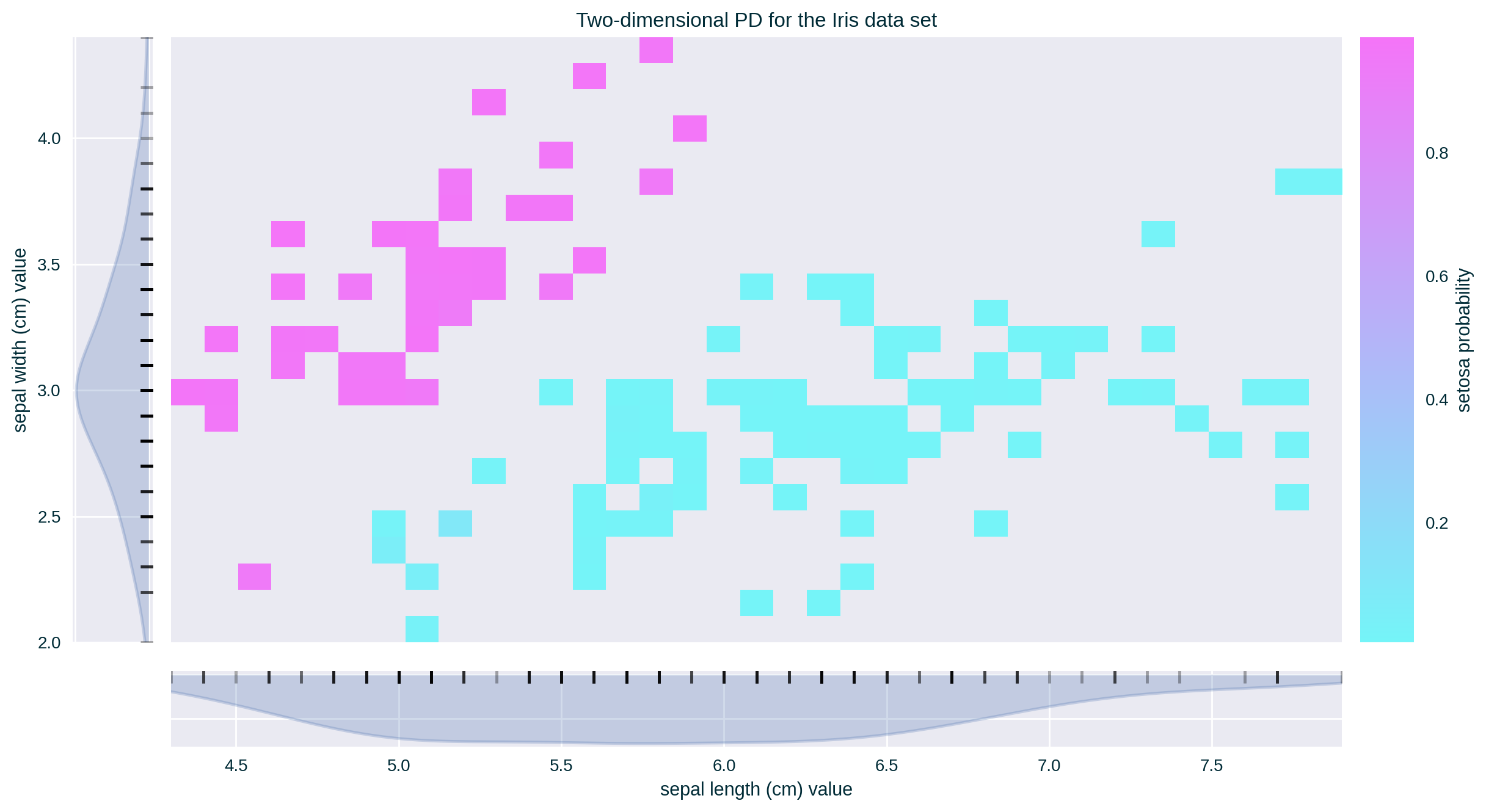
Strict ME for Two (Numerical) Features

Strict ME for Crisp Classifiers

Relaxed ME

Relaxed ME with Standard Deviation

Case Studies & Gotchas!

Feature Correlation

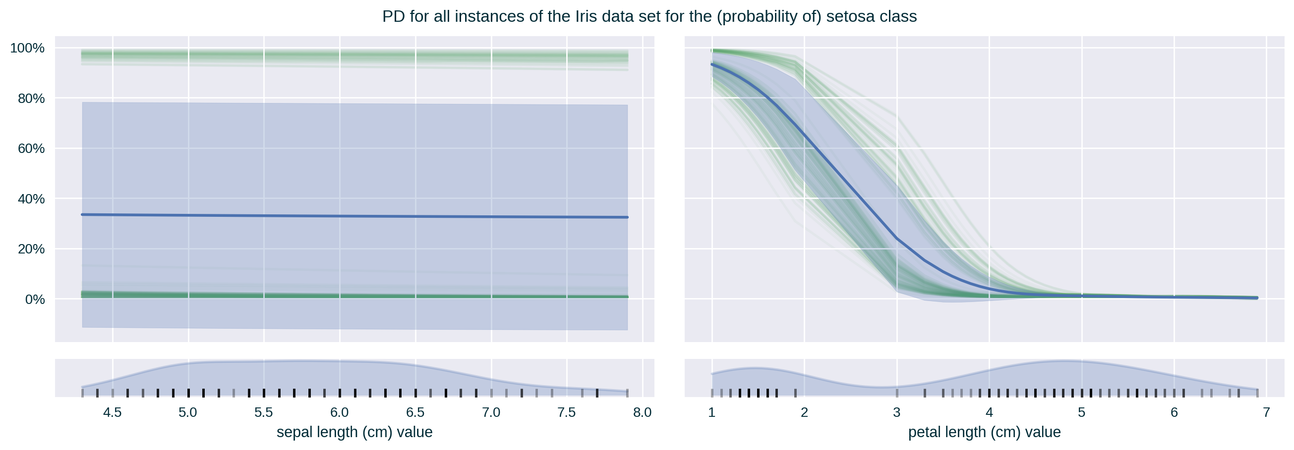
Feature Correlation    

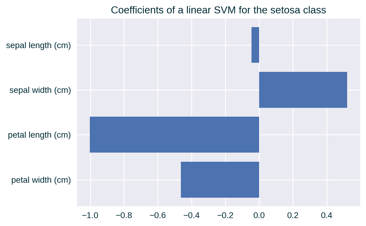
Feature Correlation    

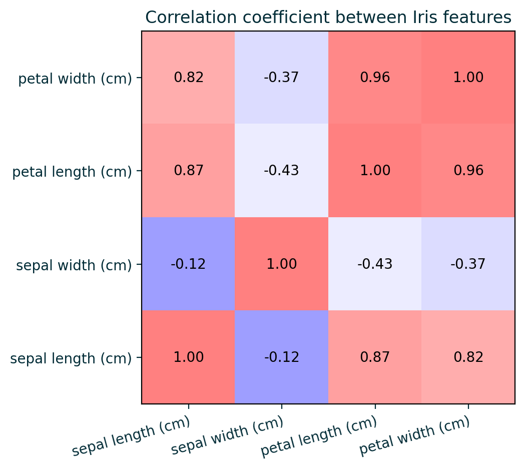
Feature Correlation    

• ME reports feature influence, but beacause of averaging only similar points the measurement gets distorted by feature correlation, therefore reporting the combined effect
• Remember that we are working with conditional distributions
• In this example, feature #1 (sepal length) – whose coefficient is close to 0 (-0.06) – shows strong influence, whcih is due to it being heavily correlated (0.87) with feature #3 (petal length) – whose coefficient has the largest magnitude (close to -1.0)
• PD, which is largely immune to this effect, does not display this behaviour

Properties

Pros    

• Easy to generate and interpret
• Based on real data

Cons    

• Assumes feature independence, which is often unreasonable and heavily biases the influence measurements
• May be unreliable for certain values of the explained feature when there is a low number of data points with that value (strict) or in a relevant bin (relaxed); this impacts the reliability of influence estimates (average perdiction of the explained model for that value or range of values)
• Reliability of estimates can only be communicated by displaying a rug plot or distribution of instances per value or bin
• Diversity (heterogeneity) of the model’s behaviour for each particular value or bin can only be communicated by prediction variance
• Limited to explaining two feature at a time

Caveats    

• The measurements may be sensitive to different binning approaches for relaxed ME
• Computational complexity: \(\mathcal{O} \left( n \right)\), where \(n\) is the number of instances in the designated data set

Further Considerations

Related Techniques

Accumulated Local Effect (ALE)

    An evolved version of (relaxed) ME that is less prone to being affected by feature correlation. It communicates the influence of a specific feature value on the model’s prediction by quantifying the average (accumulated) difference between the predictions at the boundaries of a (small) fixed interval around the selected feature value (Apley and Zhu 2020). It is calculated by replacing the value of the explained feature with the interval boundaries for instances found in the designated data set whose value of this feature is within the specified range.

Related Techniques    

Individual Conditional Expectation (ICE)

    It communicates the influence of a specific feature value on the model’s prediction by fixing the value of this feature across a designated range for a selected data point (Goldstein et al. 2015). It is an instance-focused (local) “variant” of Partial Dependence.

Related Techniques    

Partial Dependence (PD)

    It communicates the average influence of a specific feature value on the model’s prediction by fixing the value of this feature across a designated range for a set of instances. It is a model-focused (global) “variant” of Individual Conditional Expectation, which is calculated by averaging ICE across a collection of data points (Friedman 2001).

Implementations

Python	R
N/A	DALEX

Further Reading

• Interpretable Machine Learning book
• Explanatory Model Analysis book

Bibliography

Apley, Daniel W, and Jingyu Zhu. 2020. “Visualizing the Effects of Predictor Variables in Black Box Supervised Learning Models.” Journal of the Royal Statistical Society: Series B (Statistical Methodology) 82 (4): 1059–86.

Friedman, Jerome H. 2001. “Greedy Function Approximation: A Gradient Boosting Machine.” Annals of Statistics, 1189–1232.

Goldstein, Alex, Adam Kapelner, Justin Bleich, and Emil Pitkin. 2015. “Peeking Inside the Black Box: Visualizing Statistical Learning with Plots of Individual Conditional Expectation.” Journal of Computational and Graphical Statistics 24 (1): 44–65.